Lab 7 - Census 2000

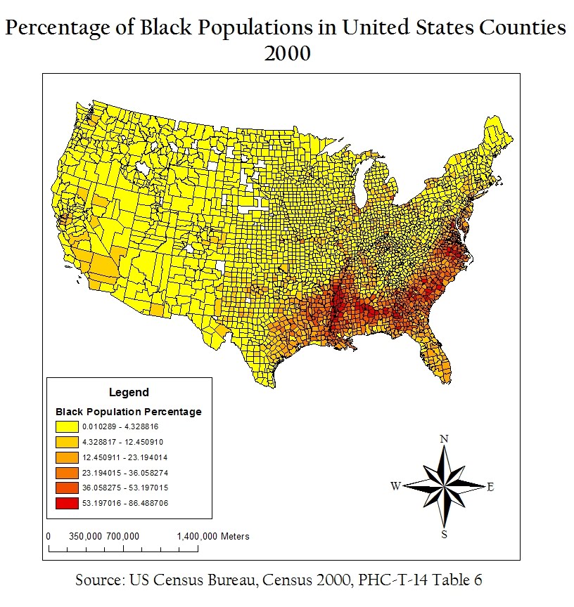
As can be seen in the “Percentage of Black Populations in United States Counties, 2000” map, black populations have a high concentration compared to other populations in the southeastern U.S. States like Mississippi, South Carolina, and Virginia have many counties with 53-86% African-Americans. Most of the rest of the United States has below 5% African-Americans represented in the populations of their counties.

In “Percentage of Asian Populations in United States Counties, 2000,” Asians have a large presence in counties on the West Coast, specifically around Seattle and San Francisco, and around some of the Northeast around New York City. What I find interesting is that no county has a population of more than 47% Asian, which is surprising considering that at many places, like UCLA, Asians are no longer a minority.

The Census Bureau has the option of “Some Other Race” as a write-in entry. For example, many people who classify themselves as multiracial, interracial, or Hispanic/Latino include themselves in the “Some Other Race” category. In 2000, 97% of the respondents who declared themselves as “Some Other Race” were Hispanic or Latino. Interestingly, only 43% of Hispanics of Latinos placed themselves in the category of “Some Other Race.” Counties in Washington, California, Texas, and New Mexico have large concentrations of people who classified themselves as “Some Other Race,” whereas most of the rest of the U.S. has less than 2% of “Some Other Race.”

These maps from the 2000 Census indicate that most minorities tend to live by some coast, whether that be near the Pacific Ocean, the Gulf of Mexico, or the Atlantic Ocean. In the middle of America, Asian, Black and “Some Other Race” do not have a high presence. This is most likely because minorities who immigrate to the United States center around major cities and ports which are generally on the edges of the U.S.

GIS is a great tool to use to display so many different types of information. I am always so excited after I have made a map that I have to show it to all of my friends. The ability to show useful information to an audience that is easy to understand is a priceless asset that GIS has imbedded in itself.

Lab 6 - DEMs in ArcGIS

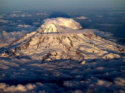
Since we were working with digital elevation models (DEMs) for this lab, I decided to choose an area with a drastic changes in elevation: Mount Rainier in Washington. Mount Rainier is one of the most dangerous volcanoes in the world and is the highest mountain in the state of Washington.

The geographic coordinate system used in the DEM is the GCS North American 1983.

The extent information for this area is:

Top: 46.96°

Left: -121.98°

Right: -121.51°

Bottom: 46.69°

The following map shows a color-ramped DEM layered above a hillshade model:

This next map shows the slope of the area around Mount Rainier in degrees:

The following map is an aspect map, which shows the direction of the slope:

This last model is a 3-D image of Mount Rainier:

 

Lab 5 - Map Projections in ArcGIS

The perfect map would be an exact representation of the real world; this would occur by having the ratio of the distances between any two points be the same on the map and in real life. However, this representation is not possible when portraying the spheroid world on a flat surface. There are three map projections that preserve some aspect of real life: equal area, equidistant, and conformal projections. In each map, I measured the distance from Washington, D.C. to Kabul in miles. The most accurate distance is using the Geographic Coordinate Systems, and is measured at around 6932 miles.

Equal area projections, as shown in the Goode’s Homolosine Land map and the Mollweide map, preserve area. In other words, the area on land is represented through the same ratio of area on the map. The Goode’s Homolosine Land map reported a distance of 9986 miles from Washington, D.C. to Kabul, while the Mollweide map reported a distance of 7926 miles. The Good Homolosine Land map’s distance is over 3000 miles off from the actual distance and the Mollweide map’s distance is just under 1000 miles off. Since the area is preserved and not the distance, the distance reported is clearly exaggerated in equal area projections.

Conformal projections, as shown in the Stereographic and Mercator maps, preserve shape and angles. Conformal projections are mainly used to represent a local area. To be considered conformal, the angles at any two lines on the map are the same as the angles in real life. The Stereographic map reported a distance of 9878 miles from Washington, D.C. to Kabul and the Mercator map reported a distance of 10,112 miles. Both of these distances are around 3000 miles more than the GCS distance, demonstrating that distance is dramatically changed when a map is focused solely on angles.

Equidistant projections, as shown in the Azimuthal Equidistant map and the Equidistant Conic map, preserve distance among a reference line. The Azimuthal Equidistant map reported a distance of 8341 miles between Washington, D.C. while the Equidistant Conic map reported a distance of 6972 miles. Clearly, the map projection that shows the most accurate distance between the two locations is the Equidistant Conic. However, the distance is not exactly what GCS reports because the equidistance aspect of the map only refers to the distance between two specific points on a reference line.

With the dramatic differences in distance between two locations shown above, it is obvious that choosing a map projection should not be taken lightly. Your map projection should depend on what you are representing on your map, from a distance-accurate city map to a shape-accurate world map.

Lab 4 - Introducing ArcGIS

My experience with ArcGIS was generally great! I really liked getting to know the program and seeing the variety of tools that could be used. For example, creating the road as well as displaying the same thing in different ways really interested me.

ArcGIS did have a few drawbacks, though. I was using ArcMap 10 when I think the tutorial was made for an older version of ArcMap. Therefore, it took me a while to find some of the tools and buttons, and I never found ArcCatelog. In addition, I feel like it will take me a long time to really get to know the program. There is so much that you can do with it that sometimes it gets confusing what steps I should take to get to the final result.

GIS has the potential to be used in every field imaginable because of its diversity and range of use. It can be helpful in determining so many things regarding distribution, location, and relationships. GIS will likely become a staple in companies and even in lower-level education.

The pitfalls of GIS include its complicated nature. Unless, like this lab, you are given step by step instructions on how to make map and how to manipulate the data, it will take a while to learn how to do it on your own. This can make it difficult to make GIS available to the masses as a viable form of analyzing data.

Lab 3 - Neogeography

View Semester at Sea Fall 2012 in a larger map

Neogeography is very useful because one can share practically anything about anywhere to anyone. In my case, my map  can give my friends and family a better idea of where I will be going and what I will be doing while on Semester at Sea. Being able to put in pictures and videos is a great way for people to visualize what the location looks like other than on a map and can give great background information. Neogeography is continuing to be developed  and has so much potential in our technology-driven world. Soon we will probably be able to integrate our My Maps into Global Positioning Systems and share the maps through those devices. One consequence of neogeography, though, is the potential lack of privacy. If everyone is making maps with their home labeled right on it and a vacation mapped out, it will not be hard to tell where they live or where they are going. People who use the My Maps feature and other neogeography tools should be sure to be careful with who they are sharing their map with.

Though there are definite benefits of neogeography, there are some pitfalls that could be worked on. For example, I had trouble embedding my YouTube video into my map. Even my friends that are computer science majors could not figure it out. Eventually I realized that I had to use a completely different code than what I was given. In addition to the video problem, drawing the line for my trip was difficult to do because there was no way to extend the line after I accidentally ended it. Technological discouragements like this are expected to happen and hopefully will soon be fixed so that neogeography can become even more advanced.

Lab 2 - USGS Topographic Map of Beverly Hills

1.  The name of the quadrangle is the Beverly Hills Quadrangle.

2.  The names of the adjacent quadrangles are Canoga Park, Van Nuys, Burbank, Topanga, Hollywood, Venice, and Inglewood.

3.  The quadrangle was first created in 1966.

4.  The horizontal datum used to create this map is the North American Datum of 1927 and the North American Datum of 1983. The vertical datum used to create this map is the National Geodetic Vertical Datum of 1929.

5.  The scale of the map is 1:24000.

6.   a) 5 cm x (1 m/ 100 cm) x 24000 = 1200 m

     5 cm on the map is equivalent to 1200 meters on the ground.

b) 5 in. x (1 ft./12 in.) x (1 mile/5280 ft.) x 24000 = 1.894

     5 inches on the map is equivalent to 1.894 miles on the ground.

c) 1 mile x (63360 in./ 1 mile) x (1/24000) = 2.64 inches

     1 mile on the ground is equivalent to 2.64 inches on the map.

d) 3 km x (100000 cm/1 km) x (1/24000) = 12.5 cm

     3 km on the ground is equivalent to 12.5 cm on the map.

7.  The contour interval on the map is 20 feet.         

8.   a) Public Affairs Building:

     34° 04’ 28” N, 118° 26’ 21” W

     34.075, -118.439°                             

b) Tip of Santa Monica Pier:

     34° 00’ 25” N, 118° 29’ 52” W

     34.007, -118.498

c) Upper Franklin Canyon Reservoir:

     34° 07’ 15” N, 118° 24’ 36” W

     34.121, -118.410

9.   a) Greystone Mansion:

     570’

     173.736 m

b) Woodlawn Cemetery:

     140’

      42.672 m

c) Crestwood Hills Park:

     750’

     228.6 m

10. The UTM zone of the map is zone 11.

11. The UTM coordinates for the lower left corner of the map are ³61.5 Easting, ³⁷63 Northing.

12.   1,000,000 square meters are contained within each cell of the UTM gridlines.

13.  

14. The magnetic declination is +14°.

15. The water flows south in the intermittent stream between the 405 freeway and Stone Canyon Reservoir because the elevation decreases as you move south along the stream.

16.  

Lab 1 - Interesting Maps!

 

“Mapping Generic Terms for Streams in the Contiguous United States” was made by Derek Watkins by using the USGS National Hydrography Dataset. It can be found on Watkins’ blog (http://derekwatkins.wordpress.com/2011/07/25/generic-stream-terms/). This map displays the varying names of streams across the United States. As can be seen from the map, these flowing waters are often called brooks in New England, bayous in Louisiana, and washes in the southwest. I find this map to be very interesting because it shows the diverse influence of language and culture in different areas of the United States. 

“World’s Most and Least Touristy Places” is a map that shows how many tourists are in certain places based on photos uploaded to Panoramio. The highest level of tourists are shown with yellow, followed by red for medium level and blue for low level of tourists. It was made by Bluemoon Interactive and can be found at http://maps.google.com/maps/mapplets?moduleurl=http://www.bluemoon.ee/~ahti/touristiness-map/touristiness-map.xml. This map interests me because when looking at the map, you have to take into account that Panoramio may not have an accurate distribution of tourists in certain areas in relation to the actual level of tourists. Regardless, I enjoy finding the high tourist levels across the world and hope that I can go to those one day in addition to the gray areas (where Panoramio has no pictures).

“Nerdy Day Trips” is a map that shows the locations of day trips for nerds on http://www.nerdydaytrips.com/. When you click on each orange icon, a window pops up telling you about the nerdy day trip. For example, in San Pedro, CA, you can visit a World War II ship and nerd out on all the history. This map interests me because of the sheer amount of nerdy day trips there are in the world and I am excited to take my fellow scholars/nerds to some of these hidden gems.